In this post I introduce a new experimental feature I am adding to goxel: procedural voxel generation.

For this I created a mini language specifically designed to describe drawing operations. Think of it as the logo language, but in 3D.

Note: this is still experimental at this point, so anything in the language could change in the future. I will try to keep this page up to date as a reference documentation.

To try it out, you need to get the last version of goxel from the github page, then use the ‘procedural’ tool, enter the code, and press ‘run’. You can use ‘auto run’ to automatically re-run the code anytime it changes.

The language is largely inspired by ContextFree language. I tried to keep it as close as possible.

Basic syntax

The smallest program (that does something) you can create is:

shape main {
    cube[]
}

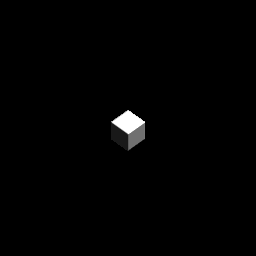
shape main is the entry point of the program and cube[] is the command used to render a cube. This program renders a 1x1x1 voxel on the screen. To make it bigger we can put adjustments inside the square brackets.

shape main {
    cube[s 9]
}

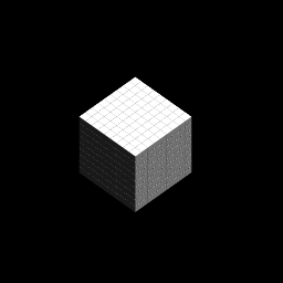
Here s 9 tells the program to make the cube 9 times bigger (s is for ‘scale’). If we wanted to scale the cube differently in x y and z we could have used the s adjustment with three arguments: cube[s 3 4 5]. Since it is common to only scale along a single axis, we can also use sx, sy and sz.

Let’s render a second cube next to the first one:

shape main {
    cube[s 9]
    cube[s 9 x 2]
}

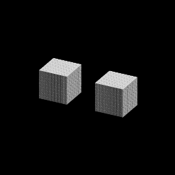
For the second cube we use two adjustments applied one after the other: s 9 to scale the cube, followed by x 2 to translate it by 2 times its size.

The adjustments are applied in order, and not commutative, so [s 9 x 2] is different from [x 2 s 9], in the first case the cube is translated by 9 voxels, in the second case only by 1.

Note the syntax of the adjustments: any values following an adjustment operation until the next operation is an argument to that operation.

Creating shapes

The basic shapes we can call are: cube, sphere, and cylinders. We can also define new shapes:

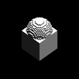
// Render a cube with a sphere on top.
shape my_shape {
    cube[]
    sphere[z 0.5]
}

shape main {
    my_shape[s 20]
}

We render the new shape just like we did for a cube. The adjustments we use in the call are applied before the shape is rendered, so in that case we render the new shape scaled 20 times. The way to understand it is that the execution of the code is linked to a context. The context define the position, size and color we are using. When we call a new shape, we duplicate the value of the current context and apply the adjustments to it before rendering the shape. It does not affect the rest of the rendering of the caller.

Recursion shapes

A shape can call itself for recurive rendering:

shape my_shape {
    cylinder[]
    my_shape [s 0.8 z 1]
}

shape main {
    my_shape[s 20]
}

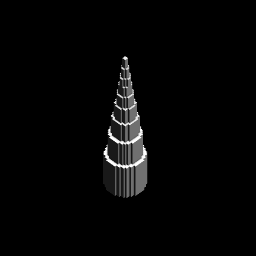
The recursion is automatically stopped when the shape becomes too small.

Loops

We can use the loop directive to create loops:

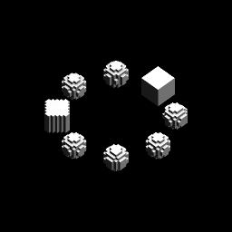
shape main {
    loop 8 [rz 45] {
        sphere[x 20 s 10]
    }
}

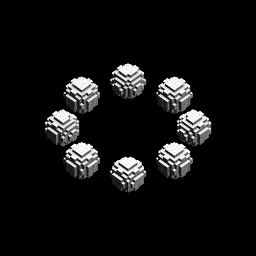
This will execute the block 8 times, each time with a context rotated 45° compared to the previous one. The adjustment only affect the block of the loop.

Expressions

We can use mathematic expression to express the adjustement arguments. The basic operations are +, -, *, /, and +-

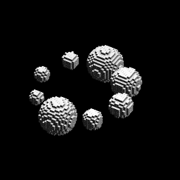
The x +- y operation returns a random value between x-y and x+y. This can be used to add some randomness to your shapes:

// Same as previous example, but the sphere
// have a random size between 4 and 16.
shape main {
    loop 8 [rz 45] {
        sphere[x 20 s 10+-6]
    }
}

Shape Rules

It is possible to give several implementations of the same shape, and let the program pick one randomly. To do this we use use shape rules:

shape my_shape
rule 4 {
    sphere[]
}
rule 1 {
    cube[]
}

shape main {
    loop 8 [rz 45] {
        my_shape[x 20 s 8]
    }
}

In this example, my_shape is most of the time a shere, but sometime a cube. The weight give the relative probabilities to use a given rule, here 4/5 chances to use the first rule, and 1/5 chance to use the second.

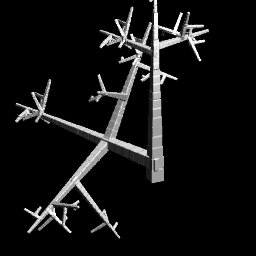
This can be used for branching effects:

shape main {
    [antialiased 1 seed 4]
    test[s 16 life 40]
}

shape test
rule 5 {
    cube[]
    test[s 0.95 z 1]
}
rule 1 {
    test[]
    test[rz 0+-180 rx 90]
}

We also see something new here: the [antialiased 1 seed 4] line apply some adjustment to the current context: antialiased 1 improves the rendering with marching cube algorithm, and seed 4 set the initial seed for the internal random function. In this example we could just have put those adjustments in the call to test.

The life 40 adjustment is here to stop the recursion after 40 iterations.

Colors

So far all the example used white color. Let see how to change that.

The color can be changed using three adjustment: light, hue and saturation, following the HSL color model. The hue varies from 0 to 360, saturation and light from 0 to 1. The initial white color corresponds to a HSL value of (0, 0, 1).

There are 3 adjustments operations to change the color: hue, sat and light. Each can take one or two arguments.

• hue x: adds the value x to the current hue. If the value gets over 360 or below 0 a modulo is applied to put it back in the range (0, 360).

• light x: x in the range [-1 +1]. If x < 0, change the light value x% toward 0. If x > 0, change the light value x% toward 1.

• sat x: x in the range [-1 +1]. If x < 0, change the saturation value x% toward 0. If x > 0, change the saturation value x% toward 1.

• hue x h change the current hue x% toward h.

• light x t change the light value x% toward t.

• sat x t change the saturation value x% toward t.

Here is a small program that render 12 spheres with different hue values:

shape main {
    [antialiased 1 sat 1 light -0.5]
    loop 12 [hue 30 rz 30] {
        sphere [s 4 x 4]
    }
}

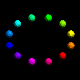
The first line sets the rendering to anti-aliased and the initial saturation and light to 1 and 0.5.

Here is a second example where we also render all the saturation values from 0 to 1. The variable $i will be explained in the next section.

shape main {
    [antialiased 1 sat 1 light -0.5]
    loop $i = 12 [z 8] {
        [sat 1 $i / 12]
        loop 12 [hue 30 rz 30] {
            sphere [x 14 s 6]
        }
    }
}

Variables

We can add variables to the code. All the variable names start with a ‘$’, so that we don’t mistake them for adjustment operations.

The first way to use variable is with the loop expression, for example:

shape main {
    [hue 180 sat 0.5]
    loop $x = 10 [] {
        cube [x $x light $x / -10]
    }
}

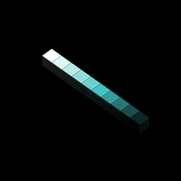
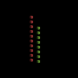
We can also use variables as argument of shapes. In that case the values need to be passed when we call the shape.

// Render n cubes
shape my_shape($n) {
    loop $n [z 2] {
        cube[]
    }
}

shape main {
    [light -0.5 sat 0.5]
    my_shape(10) []
    my_shape(8) [x 4 hue 90]
}