This post will be my attempt to explain intuitively what is Quantum Field Theory.

This idea came to me after reading two books: “QED: The Strange Theory of Light and Matter” by Richard Feynman, and “Quantum Field Theory in a Nutshell”, by A. Zee (that I only started). Both books use path integrals, but in a very different way: Feynman tells us that the particles can move anywhere they want in space and time, while Zee uses conventional ‘forward in time only’ paths but of a ‘mattress’ and not just one particle.

I tried to came up with an explanation of where the relation came from and this is the result of my thought process.

Note: this post became longer than I hoped. Here is a tldr: I am trying to show that computing the path integral of a single particle moving through space-time is similar to computing the path integral of a lattice of coupled particles connected by springs but evolving through space only. Since the relativistic paths can ‘go backward in time’, when trying to define the partial sum of the paths at a fixed ’time slice’, we need to account for the segments of paths coming from the future, making the ‘pseudo’ Lagrangian behaves similarly to the non relativistic lattice.

Big disclaimer: I am not a scientist and this is going to be extremely hand wavy. I won’t use any unit and just ignore mass and spin. For the purpose of this post, a particle has just a position. I am pretty sure the math is wrong, and maybe the whole argument doesn’t hold at all! Readers familiar with the subject can maybe tell me if this makes some sense.

Path Integral for Quantum Mechanics.

I think most people reading this have some idea of what quantum mechanic is in comparison to classical mechanics: the absolute position and speed of particles is replaced by a wave function that is related to the probability of finding the system in a given state. The Schrödinger equation then gives us the time evolution of the wave function.

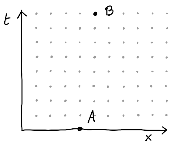
There is an other mathematically equivalent way to describe quantum mechanics, using the so-called ‘path integral’, as popularized by Feynman (though I believe the idea originally came from Dirac). I’ll present a toy model of the path integral using a discrete grid to make it easier to understand. Let’s imagine that we have a single particle in one dimension. Its position (X) can only take discrete values from 0 to -let’s say- 10. The particle starts at the position A, and we want to compute the probability of observing it at position B after a interval of time T (which we also assume to be discrete). Let’s say we have 8 time intervals:

To compute this value, we follow this algorithm:

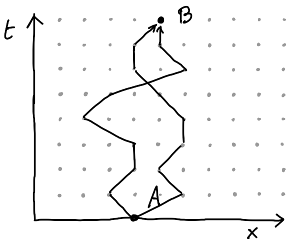
1. List all the possible paths connecting point A to the point B by picking any position for each time. Here, I’ve represented two possible paths, the actual number of paths is $10^8$:

2. For each path we compute a complex number (the amplitude) using the following algorithm: we start at the point A with the value 1 (which can also be represented as a unit vector of angle zero). Then, follow the path, and at each step consider the kinetic energy: $T \sim (dx/dt)^2$ and the potential energy: $V(x)$. Rotate the value by an angle equals to $T - V$ (the Lagrangian).

3. Finally, sum all the amplitudes for all paths. The norm of the sum gives us the probability we are looking for.

Retrieving the present time

The path integral formulation isn’t commonly discussed (at least among non-physicist) and I think it’s partly because it seems impractical to compute an infinite number of paths, but also because it’s not obvious how this relates to our normal perception of the world as some kind of state machine, going from a time $T$ to a time $ T + 1 $.

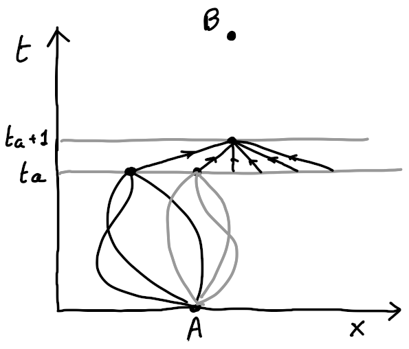
To simplify the computation of a very large number of paths, we can make the following observation: all the partial segments of a path will be summed by many paths. How can we avoid recomputing them each time? The trick is to realize that is we draw a line at a given time, all the paths will cross it at one position. If we precomputed the partial sum of all the paths below this line for all positions, we can use it at a starting value for our amplitude computation. That way, by iterating the time step by step, we only need to keep track of $N$ complex numbers, where $N$ is the number of possible position of the particle.

In this image I try to show how that works: if we’ve already computed the sums of all the paths at each point at time $t_a$, we can easily compute the sum of all the path at each point at time $t_a + 1$:

This gives us two things:

• A representation of the ‘present’ time, as a function mapping each possible state to a complex number. We can call this $\phi(x)$.

• A iteration function to evolve psi through time: $iter(\phi(x), dt) => \phi(x)$

This is not obvious and I won’t do the math, but we can show that, using the computation rule I loosely explained, the iteration function becomes the Schrodinger equation for a single particle in the limit of an infinitesimal grid.

A more complicated system

Let see quickly how the path integral would work for a system of particles. Specifically, we want to consider a one dimension lattice of particles that can each only move vertically, while being connected to their neighbor with little springs, like so:

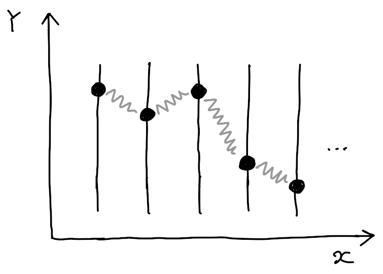
Now a single ‘state’ of the system is not just one position in $X$, but an array of positions in $Y$, one for each particle. To keep things simple, if we assume that we have 100 particles and we can only have 5 possible $Y$ values, the number of states become $ N = 5^{100} $.

The number of possible path remains $T^N = T^{5^{100}}$. We can still represent a path in a diagram, but we need to remember that each $X$ axis position now sets the position of all the particles.

The book from A. Zee almost immediately starts with the study of such a system, and then tell us that the lattice excitation can be seen as the evolution or a single relativistic particle. No explanation is given to where this relation comes from.

Here I will give a try at showing this relation. First lets see a bit how the amplitudes are computed for this system, still assuming a toy model of discrete positions and times.

The rule to compute the amplitude for a given path remains the same: we start at the beginning and for each time step we consider the start and end states, and compute the $V - T$ value to use as an angle increment. All we need is a function which given two states returns the amplitude rotation angle for the transition. This function computes the average of the potential energy for both state and subtracts kinetic energy for the difference in position of each particles.

Let see some examples of ’transitions angle’ for simple states:

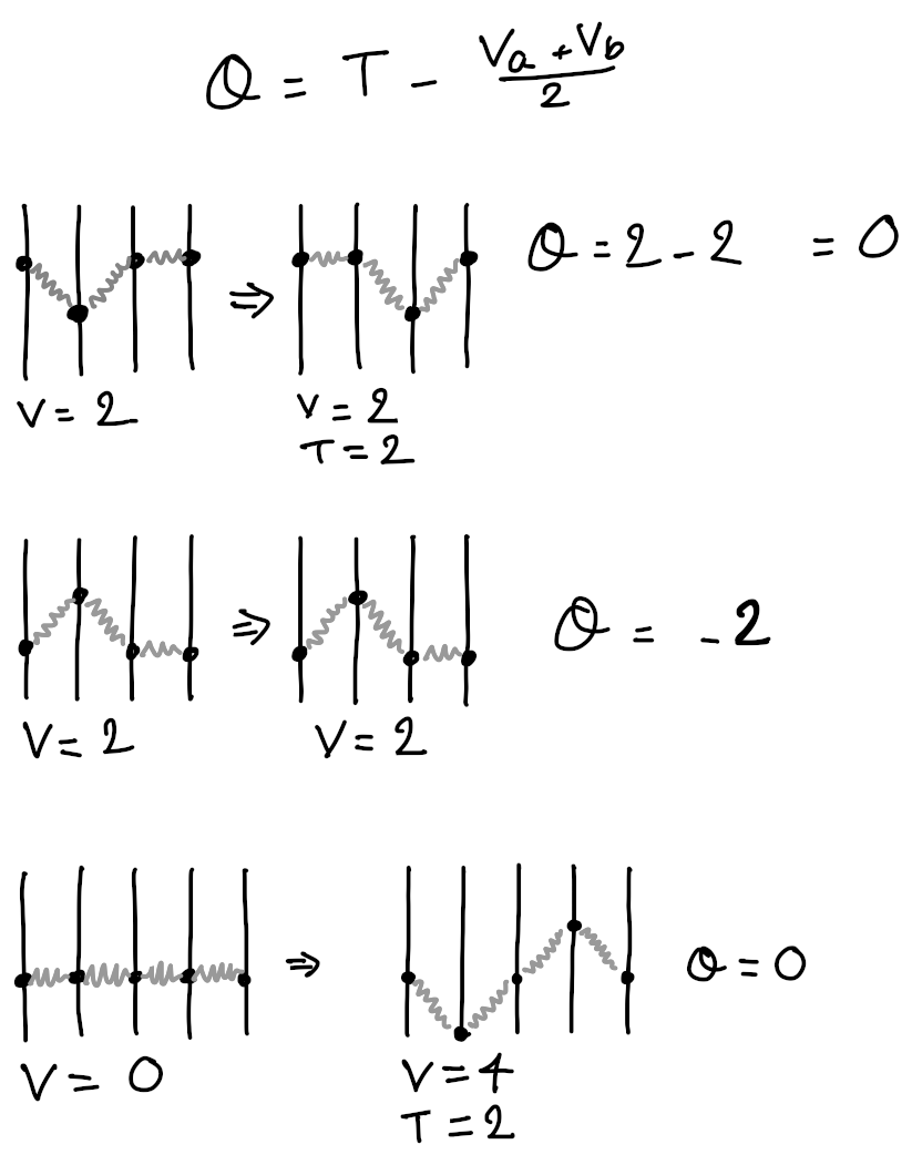
With great mathematical effort we could find and solve the Schrodinger equation for this system, but it’s not our concern here, we will stick with the path integral formulation.

Non relativistic particles

Now we can finally start to explain Quantum Field Theory. We are going to use the same framework of sum over paths, except that now the particles are relativistic: instead of moving in space with regard to time, they move in space-time with regard to their proper time $τ$(tau).

Here is how it looks like for a few samples of paths:

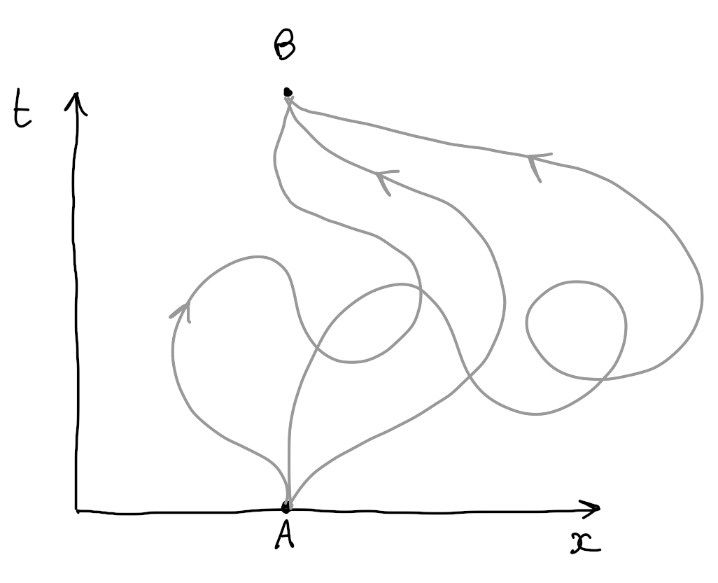
The number of paths is infinite, even if we restrict ourself to a finite grid in both space and time, since a path can take an unbounded number of steps before reaching the point B.

The other change is that the kinetic energy is no more proportional to the squared speed, but also includes a factor for the speed in time. For a single dimension particle, Instead of:

$$ T \sim (dx/dt)² $$

We use:

$$ T \sim (dx/dτ)² - (dt/dτ)² $$

The minus sign is what makes time different from space.

Can we still fix a time-line and compute a partial sum of all the paths crossing it at all the positions? Not really, because now a single path can potentially cross the fixed time line several times, in both directions, as shown here:

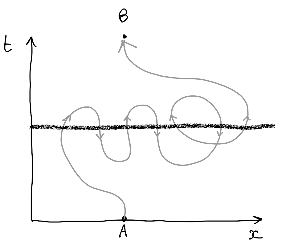
We can still try to make it work. We have to track separately the partial sum for all the paths crossing once, then all the paths crossing twice, and so on, in both directions. This can be done by assigning for each position the number of times the time line has been crossed, with a number that can be positive or negative. The wave function that used to assign a complex number to each state, like this:

$$ \phi(S) → ℂ $$

Now assigns a complex number to each possible function that assigns an integer to a state:

$$ \phi(f(S) → I) → ℂ $$

To visualise it, if we limit the number of time a path can cross the line to only 5 possible numbers $(-2, -1, 0, +1, +2)$, and we assume only 100 possible positions in the one dimension space. The number of inputs for the wave function is $N = 5^{100}$. Coincidently this is the same number we got for the non relativistic lattice of 100 particles, so we already start to see where the similarity comes from. Note that the wavefunction now keeps track of half loops even before they get connected to a valid path connecting the start and end points.

Now, we can still compute the transition angle between two of those ’extended’ states. The difference compared to before is that we have to take into account that each ‘state’ now consist of several possible paths, potentially connecting into each other.

Here are some transition angles for simple cases. Since it’s a single particle there is no potential, but the kinetic energy needs to take into account both speed in space (X) and time (T).

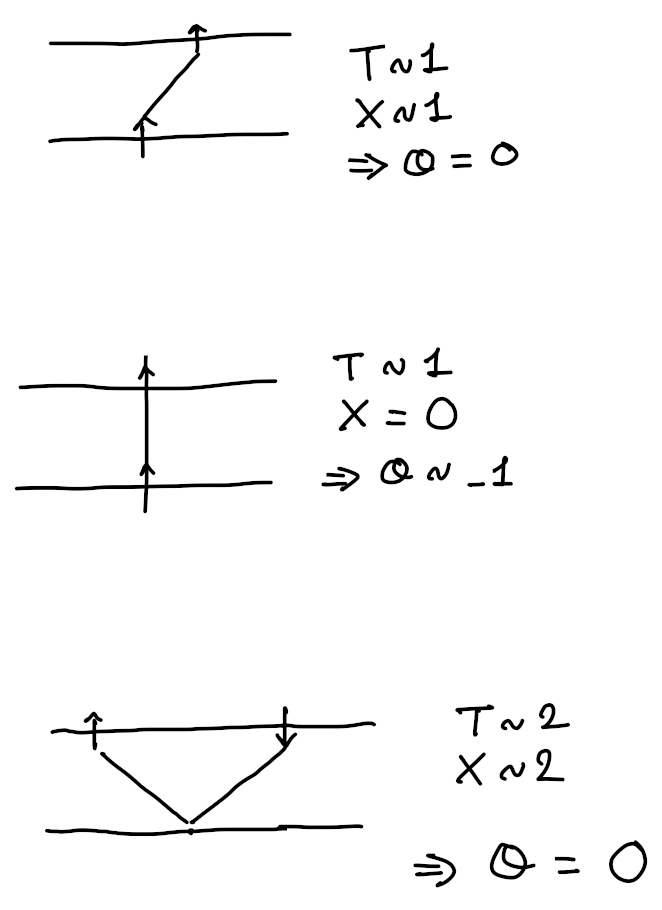
The point to note is that in the case of a path moving diagonally the angle or rotation of the amplitude is zero, while a path moving straight in time will have a negative angle. I also assume that a path turning around in time will have no impact on the amplitude.

Now if we associate the arrows directions of the path to the Y positions of our non relativistic lattice particles, we can see that the transition rules seems to relate up to a factor. Both systems, while totally different, seem to share some similarity in the way we would compute the ’time slice’ of the paths integrals.

So this was my “demonstration”. In the same way the centrifugal effect can gives rise to a “pseudo” force, the fact that the paths of a non relativistic particle can go back in time create a “pseudo” Lagrangian function similar to the one of lattice of particles.

To finish I would say once again that this explanation is not rigorous at all. One thing that bothers me (and almost make me give up on writing this) is that it’s not very clear how to handle loops and non connected paths, that would be part of the paths in the lattice model but not in the relativistic case.